AutoTSN
A systematic approach from the first ideas to a perfectly configured TSN network.
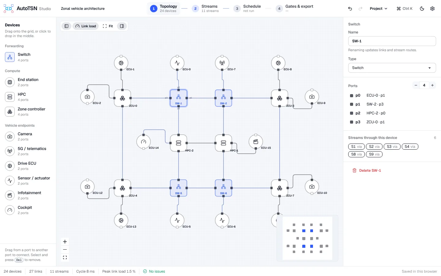
Drag switches, ECUs, cameras and computers onto the grid and connect their ports. Every port takes exactly one cable; line rates from 100 Mbit/s to 10 Gbit/s.
Four steps to a schedule
- 01
Topology
Drag switches, ECUs, cameras and computers onto the grid and connect their ports. Every port takes exactly one cable; line rates from 100 Mbit/s to 10 Gbit/s.
- 02
Streams
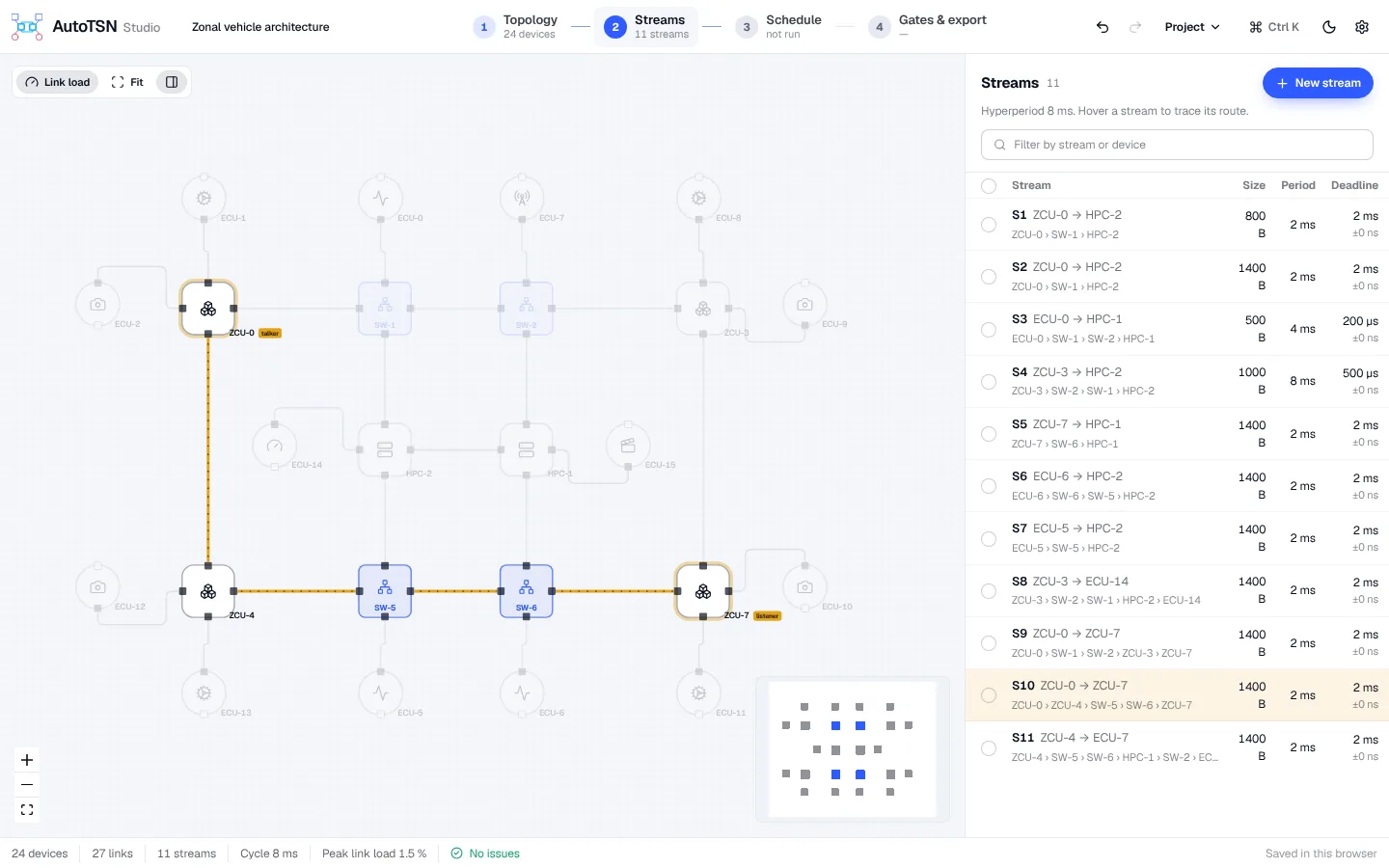
Set talker, listener, frame size, period, maximum latency and jitter. AutoTSN lists every possible route and the best achievable latency before you schedule.
- 03
Schedule
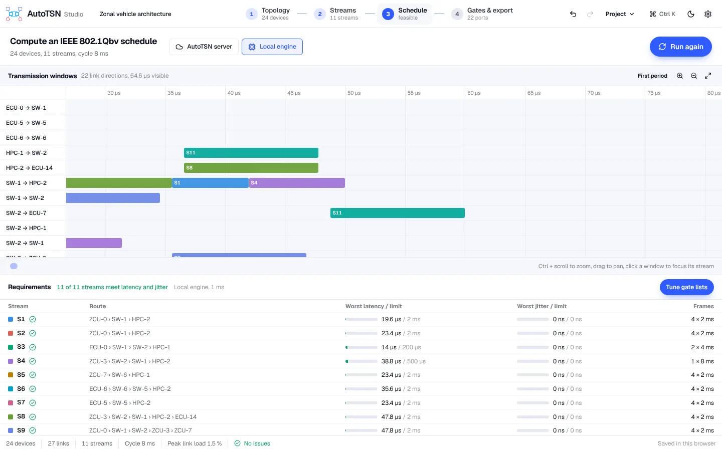
Compute the schedule on the AutoTSN server with an exact SMT solver (Z3), or instantly and offline in the browser. A Gantt chart shows every link, and a table checks latency and jitter for every stream.
- 04
Gates and export
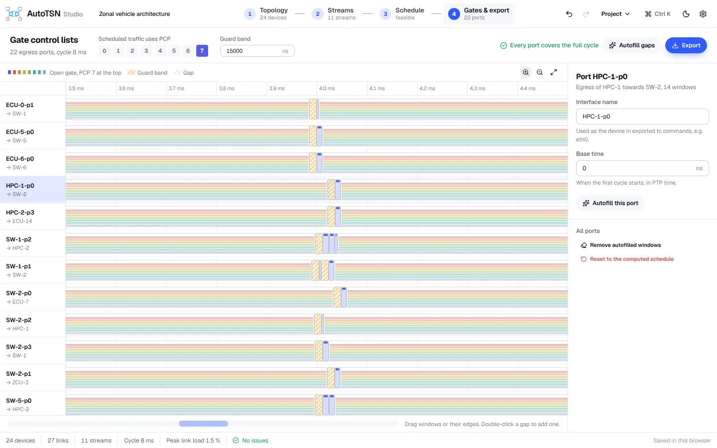
Every egress port appears with its eight gate channels. Move windows, fill gaps with best-effort windows and guard bands, and export as Linux taprio, NETCONF/YANG or JSON.
Two ways to compute
AutoTSN server
Exact SMT solver based on Z3. Finds a schedule whenever one exists, with up to 30 seconds per request.
Local engine
Zero-jitter greedy scheduler in your browser. Instant and offline, but may miss tight solutions.
Export formats
- Linux taprio
- tc commands for the time-aware priority shaper, optionally with hardware offload.
- NETCONF / YANG
- Gate parameter tables (ieee802-dot1q-sched) for NETCONF-capable bridges.
- JSON
- Every entry with start, duration and gate mask, for your own tooling.
Your projects stay saved in your browser. Only when you choose the AutoTSN server are topology and streams sent to api.autotsn.de for the computation.